


Delay Sum Beamforming
This page introduces the technique of beamforming using an array of microphones as an approach for creating a focused 'beam-like' sensitivity pattern. The simplest beamforming architecture is described, the Delay-Sum beamformer.
Introduction
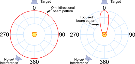
The diagram below shows the sensitivity patterns for two different microphone setups. The left hand diagram shows the pattern for an ideal omnidirectional microphone. It shows that the microphone has equal sensitivity to signals from all directions. The right hand image shows a focused sensitivity pattern aiming for maximum sensitivity in a single direction, whilst all other direction have reduced sensitivity, the goal is to create a sensitivity pattern that results in the ability to 'listen' to signals coming from a single direction.
The beamforming effect can be achieved by using a simple linear array of microphones. Such an array is illustrated below, in this case the array has three microphones. It is easy to see that the direction from which a wave front originates has an effect on the time at which the signal meets each element in the array. When arriving from -45° the signal reaches the left hand microphone first, when arriving from perpendicular to the array (called broadside) the signal reaches each microphone at the same time and when from +45° the right hand microphone receives the signal first.
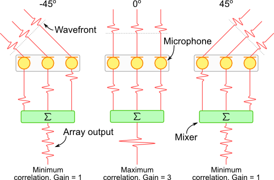
If the array's output is created by summing all microphone signals, the maximum output amplitude is achieved when the signal originates from a source perpendicular to the array; the signals arrive at the same time, they are highly correlated in time and reinforce each other. Alternatively, if the signal originates from a non-perpendicular direction, they will arrive at different times so will be less correlated and will result in a lesser output amplitude.
For a complete introduction on calculating the differences in arrival time of signals to an array see the page on Delay Calculations.
Beam Pattern
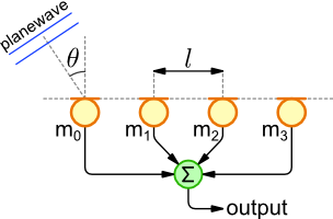
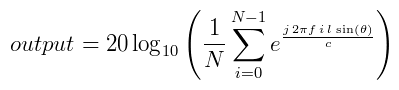
A simple calculation can be used to determine the sensitivity of a microphone array for signals coming from a particular direction. The image below shows an array with four microphones. Each array is separated by a distance l (in metres). The angle of arrival is measured from perpendicular to the array. The equation below calculates the array's gain for a single frequency f, and an arrival angle θ. c denotes the speed of sound and N is the number of microphones.
The page on Wave Summation gives a full explanation on how this equation is derived.
|
|
Note: The equation makes a few assumptions; the signal source is sufficiently far from the array that the wavefront is effectively flat, also the there is no accounting for attenuation of the signal as it travels from source to the microphones.
The gain of the array is shown in the plots below. The output is normalised to the output that would be received from a single microphone. Therefore at an angle of 0 degrees (broadside) the output amplitude is equivalent to a omnidirectional microphone, resulting in a gain of 1 (or 0 dB).
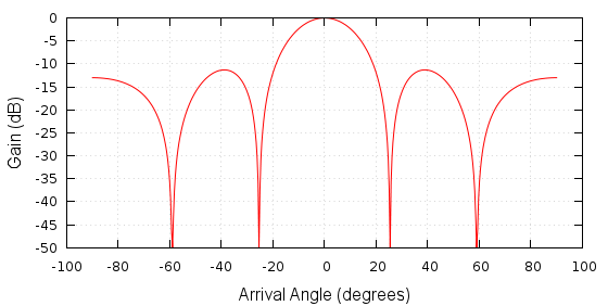
Beam Pattern, 4 Elements, 0.2m Spacing, 1kHz |
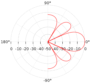
Beam Pattern in polar form |
The data for these plots was generated using the code below. It was then plotted using gnuplot. Two sets of gnuplot commands are also given below, one for the XY plot, the other for the polar plot.
beamPattern.c#include <stdio.h> #include <math.h> #define ANGLE_RESOLUTION 500 // Number of angle points to calculate int main(void) { int numElements = 4; // Number of array elements double spacing = 0.2; // Element separation in metres double freq = 1000.0; // Signal frequency in Hz double speedSound = 343.0; // m/s int a; int i; // Iterate through arrival angle points for (a=0 ; a<ANGLE_RESOLUTION ; a++) { // Calculate the planewave arrival angle double angle = -90 + 180.0 * a / (ANGLE_RESOLUTION-1); double angleRad = M_PI * (double) angle / 180; double realSum = 0; double imagSum = 0; // Iterate through array elements for (i=0 ; i<numElements ; i++) { // Calculate element position and wavefront delay double position = i * spacing; double delay = position * sin(angleRad) / speedSound; // Add Wave realSum += cos(2.0 * M_PI * freq * delay); imagSum += sin(2.0 * M_PI * freq * delay); } double output = sqrt(realSum * realSum + imagSum * imagSum) / numElements; double logOutput = 20 * log10(output); if (logOutput < -50) logOutput = -50; printf("%d %f %f %f %f\n", a, angle, angleRad, output, logOutput); } return 0; }
> gcc -lm -o beamPattern beamPattern.c
> ./beamPattern > beamPattern.dat
> gnuplot
gnuplot> call 'beamPattern.gnuplot'
The gnuplot commands below can be used for generating the two different beam pattern plots shown above.
beamPattern.gnuplotreset unset key set xlabel "Arrival Angle (degrees)" font "arial,12" set ylabel "Gain (dB)" font "arial,12" set grid lc rgbcolor "#BBBBBB" plot 'beamPattern.dat' u 2:5 w l
polar.gnuplotreset set angles degrees set polar set grid polar 30 lc rgbcolor "#999999" unset border unset param set size ratio 1 1,1 set xtics axis nomirror -50,10 unset ytics unset key set style data line set xrange[-50:50] set yrange[-50:50] set rrange[-50:0] set label 1 "0°" at graph 1.01,0.5 front set label 2 "180°" at graph -0.01,0.5 right front set label 3 "-90°" at graph 0.5,-0.03 center front set label 4 "90°" at graph 0.5,1.03 center front plot 'beamPattern.dat' u 2:5
Frequency Response
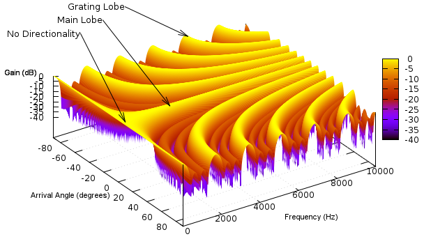
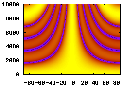
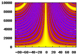
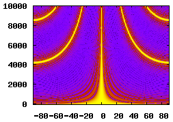
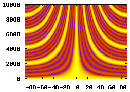
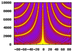
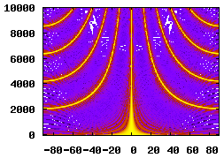
The sensitivity-plot calculation in the previous section was calculated for a single frequency. When dealing with a broadband source (such as speech) it is important to calculate an array's frequency response. The plot below shows the array's frequency response for the frequency range 0 to 10000Hz. The most noticeable features are the gain maximas where the array's output is equal to that at the perpendicular source direction. These are called grating lobes and are explained below. Their effect is a loss of directional filtering. Signal sources arriving from non-perpendicular directions will make it to the array's output in bands of frequencies.
Another interesting feature is the lack of directionality at low frequencies.
The code used to generate the data for this plot is show below. The gnuplot commands are also given.
freqResp.c#include <stdio.h> #include <math.h> #define FREQ_RESOLUTION 500 // Number of freq points to calculate #define ANGLE_RESOLUTION 500 // Number of angle points to calculate int main(void) { int numElements = 4; // Number of array elements double spacing = 0.2; // Element separation in metre double speedSound = 343.0; // m/s int f, a, i; // Iterate through arrival angle points for (f=0 ; f<FREQ_RESOLUTION ; f++) { double freq = 10000.0 * f / (FREQ_RESOLUTION-1); for (a=0 ; a<ANGLE_RESOLUTION ; a++) { // Calculate the planewave arrival angle double angle = -90 + 180.0 * a / (ANGLE_RESOLUTION-1); double angleRad = M_PI * (double) angle / 180; double realSum = 0; double imagSum = 0; // Iterate through array elements for (i=0 ; i<numElements ; i++) { // Calculate element position and wavefront delay double position = i * spacing; double delay = position * sin(angleRad) / speedSound; // Add Wave realSum += cos(2.0 * M_PI * freq * delay); imagSum += sin(2.0 * M_PI * freq * delay); } double output = sqrt(realSum * realSum + imagSum * imagSum) / numElements; double logOutput = 20 * log10(output); if (logOutput < -50) logOutput = -50; printf("%f %f %f\n", angle, freq, logOutput); } printf("\n"); } return 0; }
> gcc -lm -o freqResp freqResp.c
> ./freqResp > freqResp.dat
> gnuplot
gnuplot> call 'freqResp.gnuplot'
freqResp.gnuplotreset set xlabel "Arrival Angle (degrees)" font "arial,8" set ylabel "Frequency (Hz)" font "arial,8" set zlabel "Gain (dB)" font "arial,8" set grid lc rgbcolor "#BBBBBB" set xrange[-90:90] set yrange[0:10000] set zrange[-40:0] unset key set view 30,56,0.98 splot 'freqResp.dat' u 1:2:3 with pm3d
Microphone Spacing & Quantity
An inspection of the delay-sum equation from the Beam Pattern section reveals that the beamformer's performance is dependant on the spacing and quantity of the array's elements. The table below illustrates how changing these parameters affects the beamformer's spatial filtering performance.

|
|||

|
5 Elements, 0.04m Spacing, 0.2m Aperture |
15 Elements, 0.04m Spacing, 0.6m Aperture |
25 Elements, 0.04m Spacing, 1m Aperture |
5 Elements, 0.08m Spacing, 0.4m Aperture |
15 Elements, 0.08m Spacing, 1.2m Aperture |
25 Elements, 0.08m Spacing, 2m Aperture |
|
5 Elements, 0.16m Spacing, 0.8m Aperture |
15 Elements, 0.16m Spacing, 2.4m Aperture |
25 Elements, 0.16m Spacing, 4m Aperture |
|
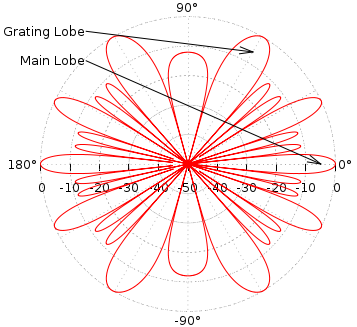
Grating Lobes
Below is a beam pattern plot for a 4 element array with 0.2m spacing at a frequency of 4kHz. The plot shows a number of extra lobes with a gain that matches the main lobe, these are called grating lobes. Grating lobes are usually unwanted as they cause the array to pick up signals from directions other than that of the main lobe without attenuation.
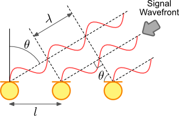
Grating lobes occur when the extra distance a signal wavefront must travel between array elements is a multiple of the signal's wavelength. In this situation, the signals received by each element are highly correlated and no signal attenuation occurs. This is illustrated in the right hand diagram below.
|
|
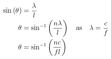
For a 1 dimensional linear array with equally spaced elements the positions of the grating lobes are easy to calculate. l is the element spacing, c is the speed of sound, f is the signal frequency and n is an integer that selects the grating lobe.
|
|
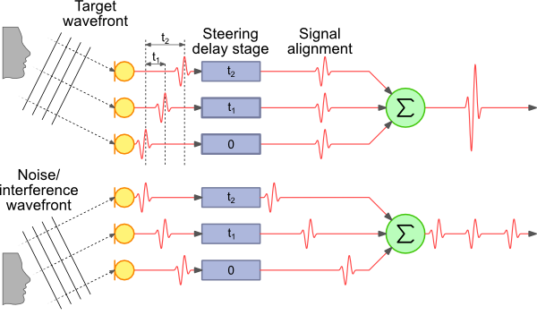
Steering
So far the main lobe of the array's sensitivity pattern has been fixed to a single direction; perpendicular to the array. A powerful feature of the beamforming array is the ability to electronically steer the beam pattern without physically moving the array. This is simply achieved by adding a delay stage to each of the array elements. The diagram below illustrates this configuration, that gives the Delay-Sum architecture its name.
The idea is very simple, add a delay to each microphone such that the signals from a particular direction are aligned before they are summed. By controlling these arrays, the main lobe direction can be steered.
One approach for implementing delay stages is described on the Fractional Delays page.
Page Revisions
| Rev Number | Date | Details |
|---|---|---|
| 1.1 | 9/3/2011 | Corrected equation in Beam Pattern section. |
| 1.2 | 10/10/2012 | Corrected axis labels on frequency response plot. |
