


FIR Filters by Windowing
The design of FIR filters using windowing is a simple and quick technique. There are many pages on the web that describe the process, but many fall short on providing real implementation details. Hopefully, this page contains all the required information to put together your own algorithm for creating low pass, high pass, band pass and band stop filters based on a number of different windows. A complete set of C functions is also provided which can be easily translated to other languages if required.
If you just want to see it all working, jump straight to the code section. All the data for the graphs on this page was generated using this code, then plotted using gnuplot.
Ideal Low Pass Filter Impulse Response
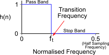
The frequency response of an ideal low pass filter is shown in the image below. The frequency axis is normalised with respect to the sampling frequency. The cut-off, or transition frequency (ft) is always between 0 and 0.5, as 0.5 represents the Nyquist frequency. As you would expect from a low pass filter, all frequencies below ft are passed, where-as all those above are stopped.
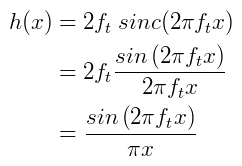
The impulse response of this ideal low pass filter is shown below, it is a sinc function. The equation is shown next to the plot. If we could create a filter with this impulse response we would have an ideal low pass filter like that shown above. A set of Gnuplot commands are also given for recreating this graph.
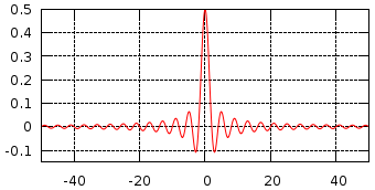
Impulse response of ideal LPF (ft=0.25) |
|
Gnuplot commands for Impulse Response (ft=0.25)
> h(x)=sin(2*pi*0.25*x)/(pi*x) > set xrange[-50:50] > set yrange[-0.15:0.5] > set samples 1000 > set grid > unset key > plot h(x) |
Below is a plot of impulse responses for different values of ft.
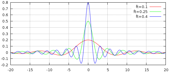
Sinc function for different values of normalised transition frequency |
Gnuplot commands
> h(x)=sin(2*pi*ft*x)/(pi*x) > set xrange[-20:20] > set samples 1000 > set grid lt rgbcolor "#BBBBBB" > plot ft=0.1, h(x) t "ft=0.1", \ > ft=0.25, h(x) t "ft=0.25", \ > ft=0.4, h(x) t "ft=0.4" |
Unfortunately it is not as easy as that. Given the non-recursive filter structure like that shown below, there are two problems with creating this ideal impulse response.
- First, the sinc function is infinite in the x direction, the ripples keep on going in both directions. However, the FIR filter only allows us to create finite impulse responses, the number of filter taps must be finite.
- Second, the impulse response is non-casual, this means an implementation would require samples from the future.
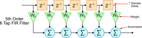
Non-Recursive, Finite Impulse Response Filter
Luckily, the solutions to these issues are quite simple. First, a window is applied to the sinc function such that only a portion of the impulse response is actually used. Secondly, the impulse response is shifted such that the filter only operates on available samples (those from the past). These techniques are demonstrated in the the following example.
Low Pass Filter Example
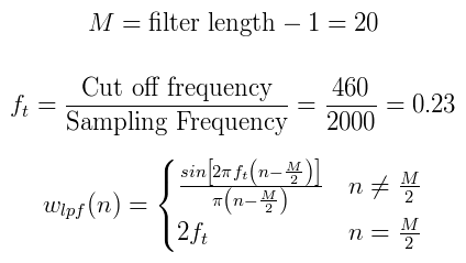
Filter weights M=20, ft=0.23
Consider the filter with the properties given below.
- Filter Type: Low Pass
- Sampling Frequency: 2000 Hz
- Cut off Frequency: 460 Hz
- Filter Length (# weights): 21
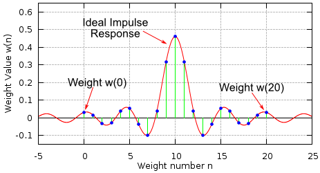
The plot to the right shows the filter weights that have been calculated using the equations below.
- M - This is the filter order, it is always equal to the number of taps minus 1
- ft - This is the normalised transition frequency.
There are 21 weights that fit on the ideal impulse response curve. It can be seen how the impulse response is effectively cropped by only using 21 weights.
Note: When calculating weight values with an odd number of weights, a divide by zero will occur at n=M/2. Therefore, based on l'Hôpital's rule, the value of 2ft is used.
The actual weight values are:
| Weight #, n | 0, 20 | 1, 19 | 2, 18 | 3, 17 | 4, 16 | 5, 15 | 6, 14 | 7, 13 | 8, 12 | 9, 11 | 10 |
|---|---|---|---|---|---|---|---|---|---|---|---|
| Weight Value w(n) | 0.030273 | 0.015059 | -0.033595 | -0.028985 | 0.036316 | 0.051504 | -0.038337 | -0.098652 | 0.039580 | 0.315800 | 0.460000 |
The frequency response for the filter is shown below. It can clearly be seen that the transition frequency occurs at the correct point, 460 Hz.
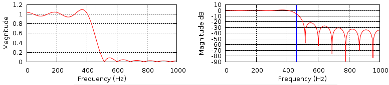
The large amount of ripple visible on the non-dB plot is due to the rather crude approach of truncating the infinite ideal impulse response. The approach that has just been used is called applying a Rectangular Window. The next section describes different window types that can decrease the ripple and improve the attenuation of the stop band.
Windowing
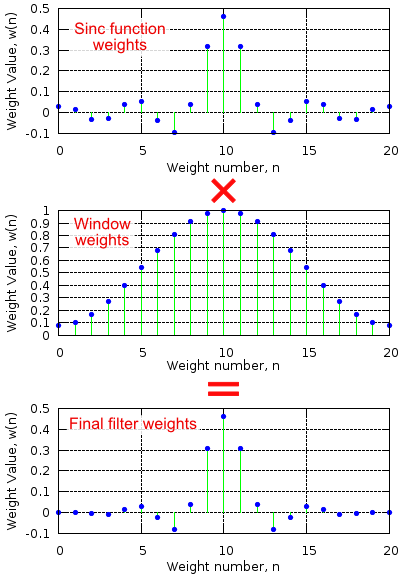
Applying a window to the sinc function weights provides extra control over the characteristics of the filter. The image to the right illustrates the process.
First, the normal sinc weights are calculated as described above. Then the window weights are calculated, in this case a Hamming Window has been used, the equation is below. The two sets of weights are multiplied together to create the final set of filter weights.
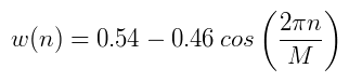
Hamming Windowing Equation
Once again, M is the order of the filter, which is equal to the filter length - 1.
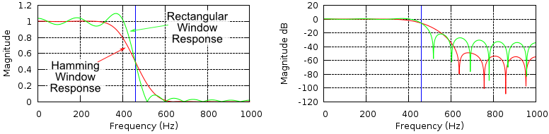
The plots below show the effect on the filter's frequency response before applying the Hamming Window (green) and after (red). The trick is to select the window type and filter length that will give a filter with the correct rate of roll-off and level of attenuation in the stop band.
Different Windows
The table below gives the equations for different window types.
| Window Type | Weight Equation |
|---|---|
| Rectangular |  |
| Bartlett | 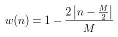 |
| Hanning | 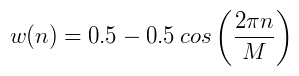 |
| Hamming | |
| Blackman | 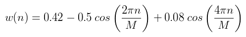 |
The image below shows the effect of different windows on the frequency response of a 28th Order (29 weights) low pass filter, with a cut-off frequency of 5000Hz and sampling frequency of 44100Hz.
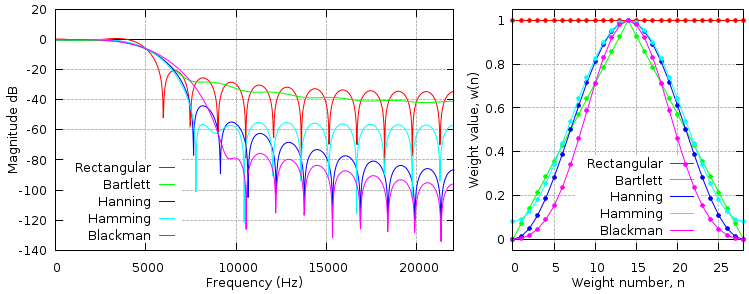
Frequency Response and Weight Values of different windows types
High Pass, Band Pass and Band Stop Filters
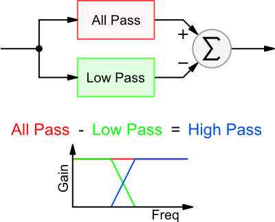
The high pass filter is made up from a low pass and an all pass filter. The image to the right demonstrates how this works. If you take an all pass filter and subtract the output of the low pass, you are left with a high pass filter.
The all pass filter is of the same order as the low pass filter. All the weight values are 0.0 apart from the centre weight which has a value 1.0. Note: This places the constraint that when creating a high pass filter in this way, the order must be even (an odd number of taps).
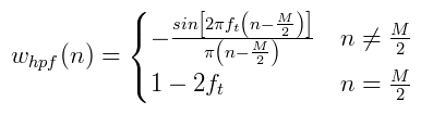
The equation for calculating the weights (before windowing) is shown below. Comparing this equation with the low pass filter it is easy to see the subtraction and the all pass filter's single 1.0 weight applied in the case of n=M/2. Windows are applied in exactly the same way as with the low pass filter.
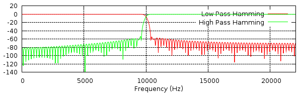
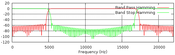
Below is a Low Pass and High Pass filter frequency response with the same transition frequency.
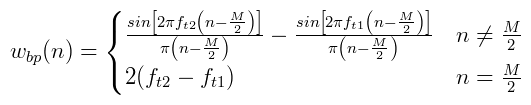
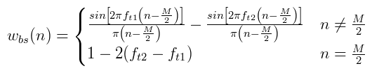
The band stop and band pass are achieved in a similar way. The equations for calculating the weights are shown below. For both band pass and band stop, the filter order needs to be even (an odd filter length). Once again, windows are applied across the weights as before.
The Kaiser Window
The Kaiser Window is specified differently to the previous windows. Rather than specifying the filter order, the amount of ripple and the transition band width are specified. The image below shows the meaning of these two parameters.
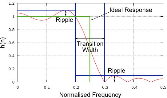
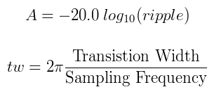
Once you have decided on the amount of ripple and transition width, using the equations below you can calculate the values for A and tw. These values can be used to calculate the filter order, M and a further parameter, β. In these equations the transition width and sampling frequency are in Hz.
|
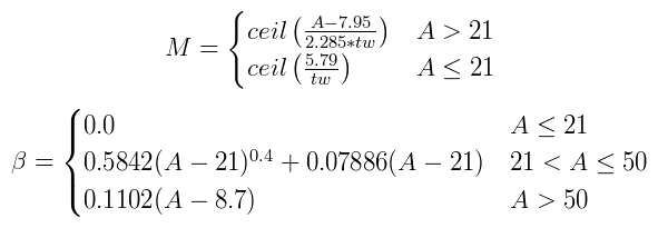
|
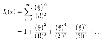
Once you have values for M and β, you can finally calculate the actual window weights. The Kaiser window equation makes use of another function I0, this is a Zeroth Order Modified Bessel Function. Although it expands to infinity, the denominator quickly becomes very large, therefore you only really need to calculate I0(x) up to around i=20.
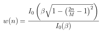
|
|
Below are some examples weights for the following Kaiser Window based low pass filter:
- Ripple: 0.01
- Cut-off Frequency: 250Hz
- Transition Window: 100Hz
- Sampling Frequency: 1000Hz
- Filter Order, M: 23
- Beta: 3.395321
| Weight #, n | 0, 23 | 1, 22 | 2, 21 | 3, 20 | 4, 19 | 5, 18 | 6, 17 | 7, 16 | 8, 15 | 9, 14 | 10, 13 | 11, 12 |
|---|---|---|---|---|---|---|---|---|---|---|---|---|
| Weight Value w(n) | -0.002896 | -0.004885 | 0.007528 | 0.010980 | -0.015463 | -0.021317 | 0.029123 | 0.039980 | -0.056254 | -0.084142 | 0.146464 | 0.448952 |
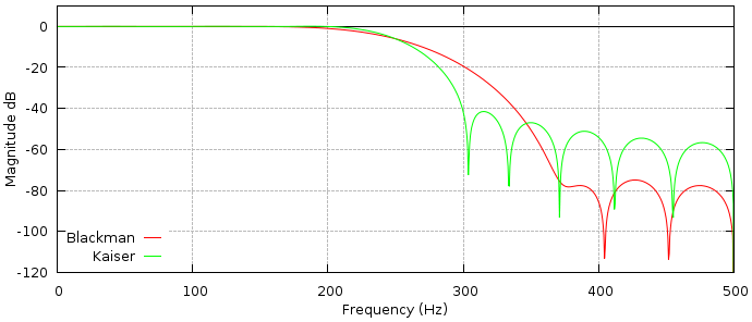
The filter's frequency response is show below, for comparison a Blackman window based filter with the same number of weights is also shown. It can be seen that the transition frequency of 250Hz is correct, as is the transition width of 100Hz.
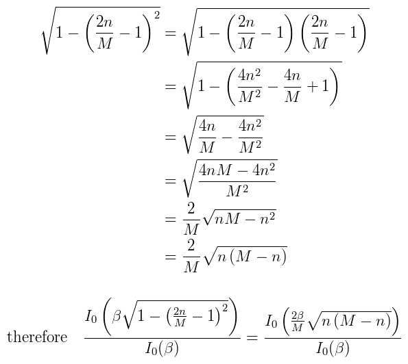
Alternate Kaiser Window Equation
Below is a rearrangement of the Kaiser Window equation.
C Code Implementation
An archive containing the source code for demonstrating all the filters and windows is linked to below.
Simply unpack and make the files as shown below. The FFTW fast Fourier transform library is used for generating the filter frequency response, this is a very standard library and should be part of any Linux distribution. It can also be used with Windows and Mac OS X.
> tar -zxf firWindowing.tar.gz
> cd firWindowing
> make
> ./filters
This will generate a set of files with extension .dat. These are frequency responses
of various filters. There is a gnuplot script to
display the data as plots.
> gnuplot
gnuplot> load 'filters.gnuplot'
Useful Links
- This page has a good set of plots for the frequency responses of different window types.
- A similar page to this, FIR filter design: The window design method.
